3 Classifiers and vector calculus
We took a first look at the core concept of machine learning in section 1.3. Then, in section 2.8.2, we examined classifiers as a special case. But so far, we have skipped the topic of error minimization: given one or more training examples, how do we adjust the weights and biases to make the machine closer to the desired ideal? We will study this topic in this chapter by discussing the concept of gradients.
NOTE The complete PyTorch code for this chapter is available at http://mng.bz /4Zya in the form of fully functional and executable Jupyter notebooks.
3.1 Geometrical view of image classification
To fix our ideas, consider a machine that classifies whether an image contains a car or a giraffe. Such classifiers, with only two classes, are known as binary classifiers. The first question is how to represent the input.
3.1.1 Input representation
The car-versus-giraffe scenario belongs to a special class of problems where we are analyzing a visual scene. Here, the inputs are the brightness levels of various points in the 3D scene projected onto a 2D image plane. Each element of the image represents a point in the actual scene and is referred to as a pixel. The image is a two-dimensional array representing the collection of pixel values at a given instant in time. It is usually scaled to a fixed size, say 224 × 224. As such, the image can be viewed as a matrix:
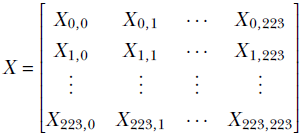
Each element of the matrix, Xi, j, is a pixel color value in the range [0,255].
Image rasterization
In the previous chapters, we have always seen a vector as the input to a machine learning system. The vector representation of the input allowed us to view it as a point in a high-dimensional space. This led to many geometric insights about classification. But here, our input is an image, which is akin to a matrix rather than a vector. Can we represent an image (matrix) as a vector?
The answer is yes. A matrix can always be converted into a vector by a process called rasterization. During rasterization, we iterate over the elements of the matrix from left to right and top to bottom, storing successive encountered elements into a vector. The result is the rasterized vector. It has the same elements as the original matrix, but they are organized differently. The length of the rasterized vector is equal to the product of the row count and column count of the matrix. The rasterized vector for the earlier matrix X has 224 × 224 = 50176 elements
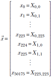
where xi ∈ [0,255] are values of the image pixels. Thus, a 224 × 224 input image can be viewed as a vector (equivalently, a point) in a 50, 176-dimensional space.
3.1.2 Classifiers as decision boundaries
We see that input images can be converted to vectors via rasterization. Each vector can be viewed as a point in a high-dimensional space. But the points corresponding to any given object or class, say giraffe or car, are not distributed randomly all over the space. Rather, they occupy a small portion subspace) in the vast high-dimensional space of inputs. This is because there is always inherent commonality in members of a class. For instance, all giraffes are predominantly yellow with a bit of black, and cars have a somewhat fixed shape. This causes the pixel values in images containing the same object to have somewhat similar values. Overall, this means points belonging to a class loosely form a cluster.
NOTE Geometrically speaking, a classifier is a hypersurface that separates the point clusters for the classes we want to recognize. This surface forms a decision boundary—the decision about which class a specific input point belongs to is made by looking at which side of the surface the point belongs to.
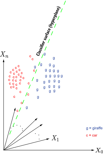
(a) Car vs. giraffe classifier
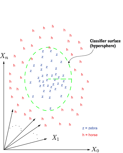
(b) Horse vs. zebra classifier
Figure 3.1 Geometric depiction of a classification problem. In the multidimensional input space, each data instance corresponds to a point. In figure 3.1a, the points marked c denote cars, and points marked g denote giraffes. This is a simple case: the points form reasonably distinct clusters, so the classification can be done with a relatively simple surface, a hyperplane. The exact parameters of the hyperplane—orientation and position—are determined via training. In figure 3.1b, the points marked h denote horses, and those marked z denote zebras. This case is a bit more difficult: the classification has to be done with a curved (nonplanar) surface, a hypersphere. The parameters of the hypersphere—radius and center—are determined via training.
Figure 3.1a shows an example of a rasterized space for the giraffe and car classification problem. The points corresponding to a giraffe are marked g, and those corresponding to a car are marked c. This is a simple case. Here, the classifier surface (aka decision boundary) that separates the cluster of points corresponding to car from those corresponding to giraffe is a hyperplane, depicted in figure 3.1a.
NOTE We often call surfaces hypersurfaces and planes hyperplanes in greater than three dimensions.
Figure 3.1b shows a more difficult example: horse and zebra classification in images. Here the points corresponding to horses are marked h and those corresponding to zebras are marked z. In this example, we need a nonlinear (curved) surface (such as a hypersphere) to separate the two classes.
3.1.3 Modeling in a nutshell
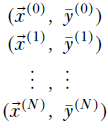
Unfortunately, in the typical scenario, we do not know the separating surface. In fact, we do not even know all the points belonging to a class of interest. All we know is a sampled set of inputs ![]() i (training inputs) and corresponding classes
i (training inputs) and corresponding classes ![]() i (the ground truth). The complete set of training inputs plus ground truth—{
i (the ground truth). The complete set of training inputs plus ground truth—{![]() i,
i, ![]() i} for a large set of i values—is called the training data. When we want to teach a baby to recognize a car, we show the baby several example cars and say “This is a car.” The training data plays the same role for a neural network.
i} for a large set of i values—is called the training data. When we want to teach a baby to recognize a car, we show the baby several example cars and say “This is a car.” The training data plays the same role for a neural network.
From only this training dataset {![]() i,
i, ![]() i} ∀i ∈ [1, n], we have to identify a good enough approximation of the general classifying surface that when presented with a random scene, we can map it to an input point
i} ∀i ∈ [1, n], we have to identify a good enough approximation of the general classifying surface that when presented with a random scene, we can map it to an input point ![]() , check which side of the surface that point lies on, and identify the class (car or giraffe). This process of developing a best guess for a surface that forms a decision boundary between various classes of interest is called modeling the classifier.
, check which side of the surface that point lies on, and identify the class (car or giraffe). This process of developing a best guess for a surface that forms a decision boundary between various classes of interest is called modeling the classifier.
NOTE The ground truth labels (![]() i) for the training images
i) for the training images ![]() i are often created manually. This process of manually generating labels for the training images is one of the most painful aspects of machine learning, and significant research effort is going on at the moment to mitigate it.
i are often created manually. This process of manually generating labels for the training images is one of the most painful aspects of machine learning, and significant research effort is going on at the moment to mitigate it.
As indicated in section 1.3, modeling has two steps:
-
Model architecture selection: Choose the parametric model function ϕ(
 ;
;  , b). This function takes an input vector and emits the class y. It has a set of parameters , b, which are unknown at first. This function is typically chosen from a bank of well-known functions that are tried and tested; for simple problems, we may choose a linear model, and for more complex problems, we choose nonlinear models. The model designer makes the choice based on their understanding of the problem. Remember, at this point the parameters are still unknown—we have only decided on the function family for the model.
 -
Model training: Estimate the parameters
, b such that ϕ emits the known correct output (as closely as possible) on the training data inputs. This is typically done via an iterative process. For each training data instance i, we evaluate yi = ϕ(i ;, b). This emitted output is compared with the corresponding known outputs ȳi. Their difference, ei = ||yi − ȳi||, is called the training error. The sum of training errors over all training data is the aggregate training error. We iteratively adjust the parameters , b such that the aggregate training error keeps going down. This means at each iteration, we adjust the parameters so the model output yi moves a little closer to the target output ȳi for all i. Exactly how to adjust the parameters to reduce the error forms the bulk of this chapter and will be introduced in section 3.3.
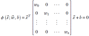
The function ϕ(![]() ;
; ![]() , b) represents the decision boundary hypersurface. For example, in the binary classification problem depicted in figure 3.1, ϕ(
, b) represents the decision boundary hypersurface. For example, in the binary classification problem depicted in figure 3.1, ϕ(![]() ;
; ![]() , b) may represent a plane (shown by the dashed line). Points on one side of the plane are classified as cars, while points on the other side are classified as giraffes. Here,
, b) may represent a plane (shown by the dashed line). Points on one side of the plane are classified as cars, while points on the other side are classified as giraffes. Here,
ϕ(![]() ;
; ![]() , b) =
, b) = ![]() T
T![]() + b
+ b
From equation 2.14 we know this equation represents a plane.
In figure 3.1b, a good planar separation does not exist—we need a nonlinear separator, such as the spherical separator shown with dashed lines. Here,
This equation represents a sphere.
It should be noted that in typical real-life cases, the separating surface does not correspond to any known geometric surface (see figure 3.2). But in this chapter, we will continue to use simple examples to bring out the underlying concepts.
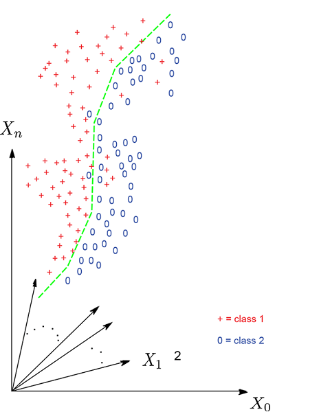
Figure 3.2 In real-life problems, the surface is often not a well-known surface like a plane or sphere. And often, the classification is not perfect—some points fall on the wrong side of the separator.
3.1.4 Sign of the surface function in binary classification
In the special case of binary classifiers, the sign of the expression ϕ(![]() ;
;![]() , b) representing the decision boundary has a special significance. To see this, consider a line in a 2D plane corresponding to the equation
, b) representing the decision boundary has a special significance. To see this, consider a line in a 2D plane corresponding to the equation
y + 2x + 1 = 0
All points on the line have x, y coordinate values satisfying this equation. The line divides the 2D plane into two half planes. All points on one half plane have x, y values such that y + 2x + 1 is negative. All points in the other half plane have x, y values such that y + 2x + 1 is positive. This is shown in figure 3.3. This idea can be extended to other surfaces and higher dimensions. Thus, in binary classification, once we have estimated an optimal decision surface ϕ(![]() ;
; ![]() , b), given any input vector
, b), given any input vector ![]() , we can compute the sign of ϕ(
, we can compute the sign of ϕ(![]() ;
; ![]() , b) to predict the class.
, b) to predict the class.
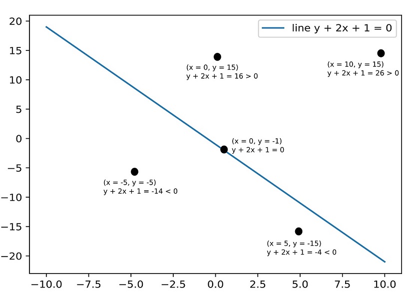
Figure 3.3 Given a point (x0, y0) and a separator y + 2x + 1 = 0, we can tell which side of the separator the point lies on from the sign of y0 + 2x0 + 1.
3.2 Error, aka loss function
As stated earlier, during training, we adjust the parameters ![]() , b so that the error keeps going down. Let’s derive a quantitative expression for this error aka loss function). Later, we will see how to minimize it.
, b so that the error keeps going down. Let’s derive a quantitative expression for this error aka loss function). Later, we will see how to minimize it.
Overall, training data consists of a set of labeled inputs (training data instances paired with known ground truths):
Now we define a loss function. On a specific training data instance, the loss function effectively measures the error made by the machine on that particular training data—input-target pair (![]() (i), y(i)). Although there are many sophisticated error functions more suitable for this problem, for now, let’s use a squared error function for the sake of simplicity (introduced in section 2.5.4). The squared error on the ith training data element is the squared difference between the output yielded by the model and the expected or target output:
(i), y(i)). Although there are many sophisticated error functions more suitable for this problem, for now, let’s use a squared error function for the sake of simplicity (introduced in section 2.5.4). The squared error on the ith training data element is the squared difference between the output yielded by the model and the expected or target output:
![]()
Equation 3.1
The total loss (aka squared error) during training is
Equation 3.2
Note that this total error is not a function of any specific training data instance. Rather, it is the overall error over the entire training data set. This is what we minimize by adjusting ![]() and b. To be precise, we estimate the
and b. To be precise, we estimate the ![]() and b that will minimize L(
and b that will minimize L(![]() , b).
, b).
3.3 Minimizing loss functions: Gradient vectors
The goal of training is to estimate the weights and bias parameter ![]() , b that will minimize L. This is usually done by an iterative process. We start with random values of
, b that will minimize L. This is usually done by an iterative process. We start with random values of ![]() , b and adjust these values so that the loss L(
, b and adjust these values so that the loss L(![]() , b) = E2(
, b) = E2(![]() , b) declines rapidly. Doing this many times is likely to take us close to the optimal values for
, b) declines rapidly. Doing this many times is likely to take us close to the optimal values for ![]() , b. This is the essential idea behind the process of training a model. It is important to note that we are minimizing the total error: this prevents us from over-indexing on any particular training instance. If the training data is a well-sampled set, the parameters
, b. This is the essential idea behind the process of training a model. It is important to note that we are minimizing the total error: this prevents us from over-indexing on any particular training instance. If the training data is a well-sampled set, the parameters ![]() , b that minimize loss over the training dataset will also work well during inferencing.
, b that minimize loss over the training dataset will also work well during inferencing.
How do we “adjust” ![]() , b so that the value of loss L = E2 declines? This is where gradients come in. For any function L(
, b so that the value of loss L = E2 declines? This is where gradients come in. For any function L(![]() , b), the gradient with respect to
, b), the gradient with respect to ![]() , b—that is, ∇
, b—that is, ∇![]() , bL(
, bL(![]() , b)—indicates the direction along which the maximum change in L occurs. The gradient is the analog of a derivative in 1D calculus. Intuitively, going down along the direction of the gradient of a function seems like the best strategy for minimizing the function value.
, b)—indicates the direction along which the maximum change in L occurs. The gradient is the analog of a derivative in 1D calculus. Intuitively, going down along the direction of the gradient of a function seems like the best strategy for minimizing the function value.
Geometrically speaking, if we start at an arbitrary point on the surface corresponding to L(![]() , b) and move along the direction of the gradient ∇
, b) and move along the direction of the gradient ∇![]() , bL(
, bL(![]() , b), we will go toward the minimum at the fastest rate (this is discussed in detail throughout the rest of this section). Hence, during training, we iteratively move toward the minimum by taking steps along ∇
, b), we will go toward the minimum at the fastest rate (this is discussed in detail throughout the rest of this section). Hence, during training, we iteratively move toward the minimum by taking steps along ∇![]() , bL(
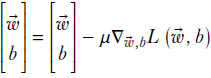
, bL(![]() , b). Note that the gradient is with respect to weights, not the input. The overall algorithm is shown in algorithm 3.2.
, b). Note that the gradient is with respect to weights, not the input. The overall algorithm is shown in algorithm 3.2.
Algorithm 3.2 Training a supervised model (overall idea)
Initialize ![]() , b with random values
, b with random values
while L(![]() , b) > threshold do
, b) > threshold do
Recompute L on new ![]() , b.
, b.
end while
![]() * ←
* ← ![]() , b* ← b
, b* ← b
-
In each iteration, we are adjusting
, b along the gradient of the error function. We will see in section 3.3 that this is the direction of maximum change for L. Thus, L is reduced at a maximal rate. -
μ is the learning rate: larger values imply longer steps, and smaller values imply shorter steps. The simplest approach, outlined in algorithm 3.2, takes equal-sized steps everywhere. In later chapters, we will study more sophisticated approaches where we try to sense how close to the minimum we are and vary the step size accordingly:
-
We take longer steps when far from the minimum, to progress quickly.
-
We take shorter steps when near the minimum, to avoid overshooting it.
-
-
Mathematically, we should keep iterating until the loss becomes minimal (that is, the gradient of the loss is zero). But in practice, we simply iterate until the accuracy is good enough for the purpose at hand.
3.3.1 Gradients: A machine learning-centric introduction
In machine learning, we model the output as a parametric function of the inputs. We define a loss function that quantifies the difference between the model output and the known ideal output on the set of training inputs. Then we try to obtain the parameter values that will minimize this loss. This effectively identifies the parameters that will result in the model function emitting outputs as close as possible to the ideal on the set of training inputs.
The loss function depends on ![]() (the model inputs), ȳ (the known ideal outputs on the training data—aka ground truth), and
(the model inputs), ȳ (the known ideal outputs on the training data—aka ground truth), and ![]() (the parameters). Here only the behavior of the loss function with respect to the parameters is of interest to us, so we are ignoring everything else and denoting the loss function as a function of the parameters as L(
(the parameters). Here only the behavior of the loss function with respect to the parameters is of interest to us, so we are ignoring everything else and denoting the loss function as a function of the parameters as L(![]() ).
).
NOTE For the sake of brevity, here we use the symbol w to denote all parameters—weight as well as bias.
The core question we are trying to answer is this: given a loss L(![]() ) and current parameter values
) and current parameter values ![]() , what is the optimal change in the parameters
, what is the optimal change in the parameters ![]() that maximally reduces the loss? Equivalently, we want to determine
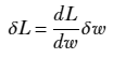
that maximally reduces the loss? Equivalently, we want to determine ![]() that will make δL = L(
that will make δL = L(![]() +
+ ![]() ) - L(
) - L(![]() ) as negative as possible. Toward that goal, we will study the relationship between the loss function L(w) and change in parameter values
) as negative as possible. Toward that goal, we will study the relationship between the loss function L(w) and change in parameter values ![]() in several scenarios of increasing complexity.1
in several scenarios of increasing complexity.1
(a) Line: L(w) = 2w + 1, dL/dw = m
(b) Parabola: L(w) = w2, dL/dw = 2w
Figure 3.4 δL in terms of δw in one dimension, illustrated with two example curves: a straight line and a parabola. In general, δL = (dL/dw) δw. To decrease loss, δw must have the opposite sign of the derivative dL/dw. In (a), this implies we always have to move left (decrease w) to decrease L. In (b), if we are in the left half (e.g., point Q), the derivative is negative, and we have to move to the right to decrease L. But if we are in the right half, the derivative is positive, and we have to move to the left to decrease L. Geometrically, this is equivalent to following the tangent “downward.”
One-dimensional loss functions
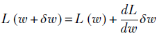
For simplicity, we begin by examining this topic in one dimension—meaning there is a single parameter w. The first example we will study is the simplest possible case: a linear one-dimensional loss function, shown in figure 3.5. A linear loss function in one dimension can be written as L(w) = mw + c. If we change the parameter w by a small amount δw, what is the corresponding change in loss δL? We have δL = L(w + δw) − L(w) = (m(w + δw)+c) − (m(w)+c) = m δw which gives us δL/δw = m, a constant. By definition, the derivative dL/dw = limδw→0 δL/δw, which leads to dL/dw = m. Thus, for the straight line L(w) = mw + c, the rate of change of L with respect to w is constant everywhere and equals the slope m. Putting all this together, we get δL = m δw = dL/dw δw.
Let’s now study a slightly more complex, non-linear but still one dimensional case—a parabolic loss function illustrated in figure 3.4. This parabola can be written as L(w) = w2. If we change the parameter w by a small amount δw, what is the corresponding change in in loss δL? We have δL = L(w + δw) − L(w) = (w + δw)2 − w2 = (2wδw + δw2). For infinitesimally small δw, δw2 becomes negligibly small and we get limδw→0 δL = limδw→0 (2wδw + δw2) = 2wδw and dL/dw = limδw→0 δL/δw = 2w. Combining all these we get the same equation as the linear case δL = dL/dw δw. Of course, in case of the straight line this expression holds for all δw while in the non-linear curves the expression holds only for small δw.
Geometrically speaking, the loss function represents a curve with the loss L(w) plotted along the Y axis against the parameter w plotted along the X axis (see figure 3.4 for examples). The tangent at any point can be viewed as the local approximation to the curve itself for an infinitesimally small neighborhood around the point. The derivative at any point represents the slope of the tangent to the curve at that point.
NOTE Equation 3.3 basically tells us that to reduce the loss value, we have to follow the tangent, moving to the right (i.e., positive δw) if the derivative is negative and moving to the left (i.e., negative δw) if the derivative is positive.
Multidimensional loss functions
If there are many tunable parameters, our loss function will be a function of many variables, which implies that we have a high-dimensional vector ![]() and a loss function L(
and a loss function L(![]() ). Our goal is to compute the change δL in L(
). Our goal is to compute the change δL in L(![]() ) caused by a small vector displacement
) caused by a small vector displacement ![]() .
.
We immediately note a fundamental difference from the one-dimensional case: the parameter change is a vector, ![]() , which has not only a magnitude denoted ||
, which has not only a magnitude denoted ||![]() || but also a direction denoted by the unit vector
|| but also a direction denoted by the unit vector ![]() . We can take a step of the same size in the w space, and the change in L(
. We can take a step of the same size in the w space, and the change in L(![]() ) will be different for different directions. The situation is illustrated in figure 3.5, which shows an example loss function L(
) will be different for different directions. The situation is illustrated in figure 3.5, which shows an example loss function L(![]() ) ≡ L(w0, w1) = 2w02 + 3w12 for two independent variables w0 and w1. Let’s examine how this loss function changes with a few concrete examples.
) ≡ L(w0, w1) = 2w02 + 3w12 for two independent variables w0 and w1. Let’s examine how this loss function changes with a few concrete examples.
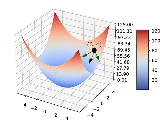
Figure 3.5 Plot for surface L(![]() ) ≡ L(w0, w1) = 2w02 + 3w12 against
) ≡ L(w0, w1) = 2w02 + 3w12 against ![]() ≡ (w0, w1). From an example point P ≡ (w0=3, w1=4, L = 66) on the surface, we can travel in many directions to reduce L. Some of these are shown byarrows. The maximum reduction occurs when we travel along the dark arrow: this happens when
≡ (w0, w1). From an example point P ≡ (w0=3, w1=4, L = 66) on the surface, we can travel in many directions to reduce L. Some of these are shown byarrows. The maximum reduction occurs when we travel along the dark arrow: this happens when ![]() is changed along
is changed along ![]() = [-12, -24]T, which is the negative of the gradient of L(
= [-12, -24]T, which is the negative of the gradient of L(![]() ) at P.
) at P.
Suppose we are at ![]() . The corresponding value of L(
. The corresponding value of L(![]() ) is 2 ∗ 32 + 3 ∗ 42 = 66. Now, suppose we undergo a small displacement from this point:
) is 2 ∗ 32 + 3 ∗ 42 = 66. Now, suppose we undergo a small displacement from this point: ![]() . The new value is L(
. The new value is L(![]() +
+ ![]() ) = L(3.0003, 4.0004) = 2 ∗ 3.00032 + 3 ∗ 4.00042 ≈ 66.0132066. Thus this displacement vector
) = L(3.0003, 4.0004) = 2 ∗ 3.00032 + 3 ∗ 4.00042 ≈ 66.0132066. Thus this displacement vector ![]() causes a change δL = 66.01320066 – 66 = 0.01320066 in L.
causes a change δL = 66.01320066 – 66 = 0.01320066 in L.
On the other hand, if the displacement is ![]() , we get L(
, we get L(![]() +
+ ![]() ) = L(3.0004, 4.0003) = 2 ∗ 3.00042 + 3 ∗ 4.00032 ≈ 66.0120006. Thus, this displacement causes a change δL = 66.0120006 − 66 = 0.0120006 in L. The displacement
) = L(3.0004, 4.0003) = 2 ∗ 3.00042 + 3 ∗ 4.00032 ≈ 66.0120006. Thus, this displacement causes a change δL = 66.0120006 − 66 = 0.0120006 in L. The displacement ![]() and
and ![]() have the same length
have the same length ![]() but different directions. The change they cause to the function value is different. This exemplifies our thesis that in multivariable loss function, the change in the loss function depends not only on the magnitude but also on the direction of the displacement in the parameter space.
but different directions. The change they cause to the function value is different. This exemplifies our thesis that in multivariable loss function, the change in the loss function depends not only on the magnitude but also on the direction of the displacement in the parameter space.
What is the general relationship between the displacement vector ![]() in the parameter space and the overall change in loss L(
in the parameter space and the overall change in loss L(![]() )? To examine this question, we need to know what a partial derivative is.
)? To examine this question, we need to know what a partial derivative is.
Partial derivatives
The derivative dL/dw of a function L(w) indicates the rate of change of the function with respect to w. But if L is a function of many variables, how does it change if only one of those variables is changed? This question leads to the notion of partialderivatives.
The partial derivative of a function of many variables is a derivative taken with respect to exactly one variable, treating all other variables as constants. For instance, given L(![]() ) ≡ L(w0, w1) = 2w02 + 3w12, the partial derivatives with respect to w0 , w1 are
) ≡ L(w0, w1) = 2w02 + 3w12, the partial derivatives with respect to w0 , w1 are
Total change in a multidimensional function
Partial derivatives estimate the change in a function if a single variable changes and the others stay constant. How do we estimate the change in a function’s value if all the variables change together?
The total change can be estimated by taking a weighted combination of the partial derivatives. Let ![]() and
and ![]() denote the point and the displacement vector, respectively:
denote the point and the displacement vector, respectively:
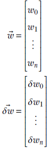
Then
Equation 3.4
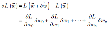
Equation 3.4 essentially says that the total change in L is obtained by adding up the changes caused by displacements in individual variables. The rate of change of L with respect to the change in wi only is ∂L/∂wi. The displacement along the variable wi is δwi. Hence, the change caused by the ith element of the displacement is ∂L/∂wi δwi— this follows from equation 3.3. The total change is obtained by adding the changes caused by individual elements of the displacement vector: that is, summing over all i from 0 to n. This leads to equation 3.4. Thus equation 3.4 is simply the multidimensional version of equation 3.3.
Gradients
It would be nice to be able to represent equation 3.4 compactly. To do this, we define a quantity called a gradient: the vector of all the partial derivatives.
Given an n-dimensional function L(![]() ), its gradient is defined as
), its gradient is defined as
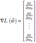
Equation 3.5
Using gradients, we can rewrite equation 3.4 as
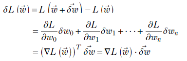
Equation 3.6
Equation 3.6 tells us that the total change, δL in L(![]() ), caused by displacement
), caused by displacement ![]() from
from ![]() in parameter space is the dot product between the gradient vector ∇L(
in parameter space is the dot product between the gradient vector ∇L(![]() ) and the displacement vector
) and the displacement vector ![]() . This is the exact multidimensional analog of equation 3.3.
. This is the exact multidimensional analog of equation 3.3.
Recall from section 2.5.6.2 that the dot product of two vectors (of fixed magnitude) attains a maximum value when the vectors are aligned in direction. This yields a physical interpretation of the gradient vector: its direction is the direction in parameter space along which the multidimensional function is changing fastest. It is the multidimensional counterpart of the derivative. This is why, in machine learning, when we want to minimize the loss function, we change the parameter values along the direction of the gradient vector of the loss function.
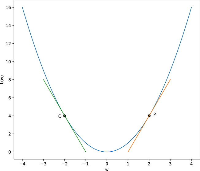
The gradient is zero at the minimum
any optimum (that is, maximum or minimum) of a function is a point of inflection. This means the function turns around at the optimum point. In other words, the gradient direction on one side of the optimum is the opposite of that on the other side. If we try to travel smoothly from positive values to negative values, we must cross zero somewhere in between. Thus, the gradient is zero at the exact point of inflection maximum or minimum). This is easiest to see in 2D and is depicted in figure 3.6. However, the idea is general: it works in higher dimensions, too. The fact that the gradient becomes zero at the optimum is often used to algebraically compute the optimum. The following example illustrates this.
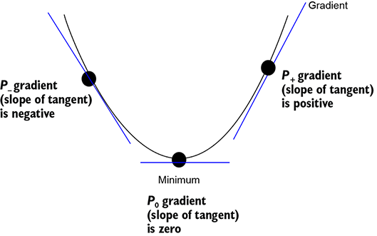
Figure 3.6 The minimum is always a point of inflection, meaning the function turns around at that point. If we consider any two points P− and P + on both sides of the minimum, the gradient is positive on one side and negative on the other. Assuming the gradient changes smoothly, it must be zero in between, at the minimum.
Consider the simple example function L(w0, w1) = √w02 + w12. Its optimum occurs when its gradient is zero:
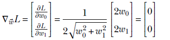
The solution is w0 = 0, w1 = 0 The function attains its minimum value at the origin, which agrees with our intuition.
3.3.2 Level surface representation and loss minimization
In figure 3.5, we plotted the loss function L(![]() ) against the parameter values
) against the parameter values ![]() . In this section, we study a different way of visualizing loss surfaces. This will lend further insight into gradients and minimization.
. In this section, we study a different way of visualizing loss surfaces. This will lend further insight into gradients and minimization.
We will continue with our simple example function from the last subsection. Consider a field L(w0, w1) = √(w02 + w12). Its domain is the infinite 2D plane defined by the axes W0 and W1. Note that the function has constant values along concentric circles centered on the origin. For instance, at all points on the circumference of the circle w02 + w12 = 1, the function has a constant function value of 1. At all points on the circumference of the circle w02 + w12 = 25, the function has a constant function value of 5. Such constant function value curves on the domain are called level contours in 2D. This is shown as a heat map in figure 3.7. The idea of level contours can be generalized to higher dimensions where we have level surfaces or level hypersurfaces. Note that while the ![]() , L(
, L(![]() ) in figure 3.5 was on an (n+1)-dimensional space (where n is the dimensionality of
) in figure 3.5 was on an (n+1)-dimensional space (where n is the dimensionality of ![]() ), the level surface/contour representation is in n-dimensional space. At any point on the domain, what is the direction along which the biggest change in the function value occurs? The answer is along the direction of the gradient. The magnitude of the change corresponds to the magnitude of the gradient. In the current example, say we are at a point (w0, w1). There exists a level contour through this point: the circle with origin at the center passing through (w0, w1). If we move along the circumference of this circle—that is, along the tangent to this circle—the function value does not change. In other words, at any point, the tangent to the level contour through that point is the direction of minimal change. On the other hand, if we move perpendicular to the tangent, maximum change in the function value occurs. The perpendicular to the tangent is known as a normal. This is the direction of the gradient. The gradient at any point on the domain is always normal to the level contour through that point, indicating the direction of maximum change in the function value. In figure 3.7, the gradients are all parallel to the radii of the concentric circles.
), the level surface/contour representation is in n-dimensional space. At any point on the domain, what is the direction along which the biggest change in the function value occurs? The answer is along the direction of the gradient. The magnitude of the change corresponds to the magnitude of the gradient. In the current example, say we are at a point (w0, w1). There exists a level contour through this point: the circle with origin at the center passing through (w0, w1). If we move along the circumference of this circle—that is, along the tangent to this circle—the function value does not change. In other words, at any point, the tangent to the level contour through that point is the direction of minimal change. On the other hand, if we move perpendicular to the tangent, maximum change in the function value occurs. The perpendicular to the tangent is known as a normal. This is the direction of the gradient. The gradient at any point on the domain is always normal to the level contour through that point, indicating the direction of maximum change in the function value. In figure 3.7, the gradients are all parallel to the radii of the concentric circles.
Recall that while training a machine learning model, we essentially define a loss function in terms of a tunable set of parameters and try to minimize the loss by adjusting (tuning) the parameters. We start at a random point and iteratively progress toward the minimum. Geometrically, this can be viewed as starting at an arbitrary point on the domain and continuing to move in a direction that minimizes the function value. Of course, we would like to progress to the minimum of the function value in as few iterations as possible. In figure 3.7, the minimum is at the origin, which is also the center of all the concentric circles. Wherever we start, we will have to always travel radially inward to reach the minimum (0,0) of the function √(w02 + w12).
In higher dimensions, level contours become level surfaces. Given any function L(![]() ) with
) with ![]() ] ∈ ℝn, we define level surfaces as L(
] ∈ ℝn, we define level surfaces as L(![]() ) = constant. If we move along the level surface, the change in L(
) = constant. If we move along the level surface, the change in L(![]() ) is minimal (0). The gradient of a function at any point is normal to the level surface through that point. This is the direction along which the function value is changing fastest. Moving along the gradient, we pass from one level surface to another, as shown in figure 3.8. Here the function is 3D: L(
) is minimal (0). The gradient of a function at any point is normal to the level surface through that point. This is the direction along which the function value is changing fastest. Moving along the gradient, we pass from one level surface to another, as shown in figure 3.8. Here the function is 3D: L(![]() ) = L(w0, w1, w2) = w02 + w12 + w22. The level surfaces w02 + w12 + w22 = constant for various values of the constant are concentric spheres, with the origin as their center. The gradient vector at any point is along the outward-pointing radius of the sphere through that point.
) = L(w0, w1, w2) = w02 + w12 + w22. The level surfaces w02 + w12 + w22 = constant for various values of the constant are concentric spheres, with the origin as their center. The gradient vector at any point is along the outward-pointing radius of the sphere through that point.
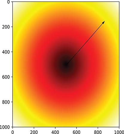
Figure 3.7 The domain of L(w0, w1) = √(w02 + w12) shown as a heat map of function values. Gradients point radially outward, as shown by the arrowed line. The intensity of the heat map changes fastest along the gradient (that is, radii). This is the direction to follow to rapidly reach lower values of the function represented by the heat map.
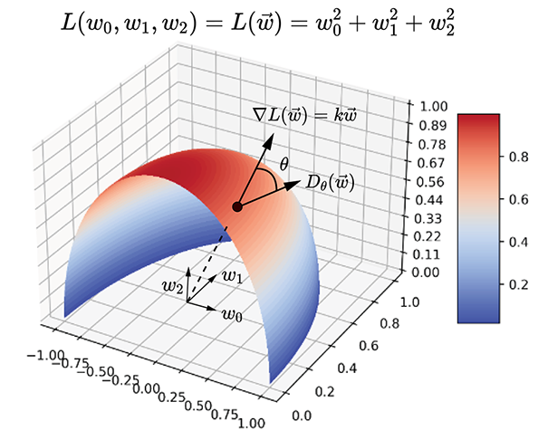
Figure 3.8 Gradient example in 3D: the function L(w0, w1, w2) = L(![]() ) = w02 + w12 + w22. The levelsurfaces L(
) = w02 + w12 + w22. The levelsurfaces L(![]() ) = constant are concentric spheres with the origin as their center. One such surface is partially shown in the diagram. ∇L(
) = constant are concentric spheres with the origin as their center. One such surface is partially shown in the diagram. ∇L(![]() ) = k[w0 w1 w2]T—the gradient points radially outward. along the gradient, we go from one level surface to another, corresponding to maximum change in L(
) = k[w0 w1 w2]T—the gradient points radially outward. along the gradient, we go from one level surface to another, corresponding to maximum change in L(![]() ). Moving along any direction orthogonal to the gradient, we stay on the same level surface (sphere), which corresponds to zero change in the function value. Dθ(
). Moving along any direction orthogonal to the gradient, we stay on the same level surface (sphere), which corresponds to zero change in the function value. Dθ(![]() ) denotes the directional derivative along the displacement direction making angle θ with the gradient. If l̂ denotes this displacement direction, Dθ(
) denotes the directional derivative along the displacement direction making angle θ with the gradient. If l̂ denotes this displacement direction, Dθ(![]() ) = ∇L(
) = ∇L(![]() ) ⋅ l̂.
) ⋅ l̂.
Another example is shown in figure 3.9. Here the function is 3D: L(![]() ) = f(w0, w1, w2) = w02 + w12. The level surfaces w02 + w12 = constant for various values of the constant are coaxial cylinders, with w2 as the axis. The gradient vector at any point is along the outward-pointing radius of the planar circle belonging to the cylinder through that point.
) = f(w0, w1, w2) = w02 + w12. The level surfaces w02 + w12 = constant for various values of the constant are coaxial cylinders, with w2 as the axis. The gradient vector at any point is along the outward-pointing radius of the planar circle belonging to the cylinder through that point.
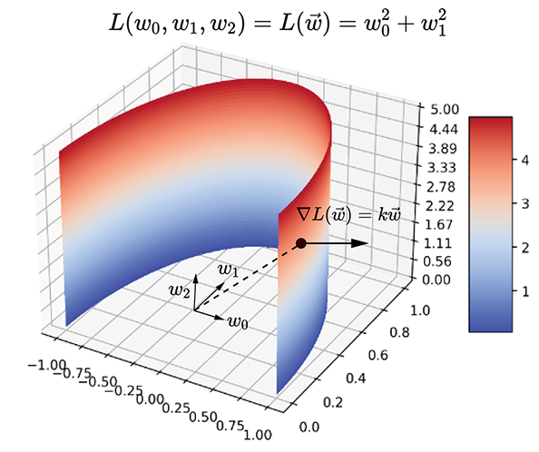
Figure 3.9 Gradient example in 3D: the function L(w0, w1, w2) = L(![]() ) = w02 + w12. The level surfaces f(
) = w02 + w12. The level surfaces f(![]() ) = constant are coaxial cylinders. One such surface is partially shown in the diagram: ∇L(
) = constant are coaxial cylinders. One such surface is partially shown in the diagram: ∇L(![]() ) = k[w0 w1 0]T. The gradient is normal to the curved surface of the cylinder along the outward radiusof the circle. Moving along the gradient, we go from one level surface to another, corresponding to themaximum change in L(
) = k[w0 w1 0]T. The gradient is normal to the curved surface of the cylinder along the outward radiusof the circle. Moving along the gradient, we go from one level surface to another, corresponding to themaximum change in L(![]() ). Moving along any direction orthogonal to the gradient, we stay on thesame level surface (cylinder), which corresponds to zero change in the function value.
). Moving along any direction orthogonal to the gradient, we stay on thesame level surface (cylinder), which corresponds to zero change in the function value.
So far, we have studied the change in loss value resulting from infinitesimally small displacements in the parameter space. In practice, the programmatic displacements undergone during parameter updates while training are small, but not infinitesimally so. Is there any way to improve the approximation in these cases? This is discussed in the following section.
3.4 Local approximation for the loss function
Equation 3.6 expresses the change δL in the loss value corresponding to displacement ![]() in the parameter space. The equation is exactly true if and only if the loss function is linear or the magnitude of the displacement is infinitesimally small. In practice, we adjust parameter values by small—but not infinitesimally small—amounts. Under these circumstances, equation 3.6 is only approximately true: the larger the magnitude of ||
in the parameter space. The equation is exactly true if and only if the loss function is linear or the magnitude of the displacement is infinitesimally small. In practice, we adjust parameter values by small—but not infinitesimally small—amounts. Under these circumstances, equation 3.6 is only approximately true: the larger the magnitude of ||![]() ||, the worse the approximation.
||, the worse the approximation.
A Taylor series offers a way to approximate a multidimensional function in the local neighborhood of any point by expressing it in terms of the displacements in the parameter space. It is an infinite series, meaning the equation is exactly true (zero approximation) only when we have summed an infinite number of terms. Of course, we cannot add an infinite number of terms with a computer program. But we can improve the accuracy of the approximation as much as we like by including more and more terms. In practice, we include at most up to the second term. Anything beyond that is redundant because the improvement is too small to be realized by the floating point system of current computers. First we will study a Taylor series in one dimension.
3.4.1 1D Taylor series recap
Suppose we are trying to describe the curve L(w) in the neighborhood of a particular point w. If we stay infinitesimally close to w, then, as described in section 3.3, we can approximate the curve with a straight line:
But in the general case, if we are describing a continuous (smooth) function in the neighborhood of a specific point, we use a Taylor series. A Taylor series allows us to describe a function in the neighborhood of a specific point in terms of the value of the function and its derivatives at that point. Doing so is relatively simple in 1D:
Equation 3.7
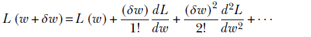
Note that the terms become progressively smaller (since they involve higher and higher powers of a small number δw). Hence, although the series goes on to infinity, in practice we entail a negligible loss in accuracy by dropping higher-order terms. We often use the first-order approximation (or, at most, second-order). Equation 3.7 can be rewritten as
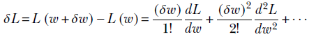
Note that the second term has (δw)2 as a factor, which is nearly zero at small values of the displacement δw. So, for really small δw, we include only the first term. Then we get δL = (δw/1!) (dL/dw), which is the same as equation 3.3. If δw is a bit larger and we want greater accuracy, we can include the second-order term. In practice, as mentioned earlier, that is hardly ever done.
A handy example of a Taylor series is the expansion of the exponential function ex near x = 0
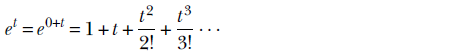
where we use the fact that dn/dxn (ex)|x = 0 = ex|x = 0 = 1 for all n.
3.4.2 Multidimensional Taylor series and the Hessian matrix
In equation 3.7, we express a function of one variable in a small neighborhood around a point in terms of the derivatives. Can we do a similar thing in higher dimensions? Yes. We simply need to replace the first derivative with the gradient. We replace the second derivative with its multidimensional counterpart: the Hessian matrix. The multidimensional Taylor series is as follows

Equation 3.8
where H(L(![]() )), called the Hessian matrix, is defined as
)), called the Hessian matrix, is defined as
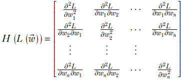
Equation 3.9
The Hessian matrix is symmetric since ![]() . Also, note that the Taylor expansion assumes that the function is continuous in the neighborhood.
. Also, note that the Taylor expansion assumes that the function is continuous in the neighborhood.
Equation 3.8 allows us to compute the value of L in a small neighborhood around point ![]() in the parameter space. If we displace from
in the parameter space. If we displace from ![]() by the vector
by the vector ![]() , we arrive at
, we arrive at ![]() +
+ ![]() . The loss there is L(
. The loss there is L(![]() +
+ ![]() ), which is expressed by equation 3.8 in terms of the loss L(
), which is expressed by equation 3.8 in terms of the loss L(![]() ) at the original point and the displacement
) at the original point and the displacement ![]() .
.

Equation 3.10
Note that the first term is same as equation 3.6 and the second term has squares of the displacement. Since the square of a small quantity is even smaller, for very small displacements, the second term disappears, and we essentially get back equation 3.6. This is called first-order approximation. For slightly larger displacements, we can include the second term, involving Hessians to improve the approximation. As stated earlier, this is hardly ever done in practice.
3.5 PyTorch code for gradient descent, error minimization,and model training
In this section, we study PyTorch examples in which models are trained by minimizing errors via gradient descent. Before we present the code, we briefly recap the main ideas from a practical point of view. Complete code for this section can be found at http://mng.bz/4Zya.)
3.5.1 PyTorch code for linear models
If the true underlying function we are trying to predict is very simple, linear models suffice. Otherwise, we require nonlinear models. Here we will look at the linear model. In machine learning, we identify the input and output variables pertaining to the problem at hand and cast the problem as generating outputs from input variables. All the inputs are represented together by the vector ![]() . Sometimes there are multiple outputs, and sometimes there is a single output. Accordingly, we have an output vector
. Sometimes there are multiple outputs, and sometimes there is a single output. Accordingly, we have an output vector ![]() or an output scalar y. Let’s denote the function that generates the output from the input vector as f: that is, y = f(
or an output scalar y. Let’s denote the function that generates the output from the input vector as f: that is, y = f(![]() ).
).
In real-life problems, we do not know f. The crux of machine learning is to estimate f from a set of observed inputs ![]() i and their corresponding outputs yi. Each observation can be depicted as a pair ⟨
i and their corresponding outputs yi. Each observation can be depicted as a pair ⟨![]() i, yi⟩. We model the unknown function f with a known function ϕ. ϕ is a parameterized function. Although the nature of ϕ is known, its parameter values are unknown. These parameter values are “learned” via training. This means we estimate the parameter values such that the overall error on the observations is minimized.
i, yi⟩. We model the unknown function f with a known function ϕ. ϕ is a parameterized function. Although the nature of ϕ is known, its parameter values are unknown. These parameter values are “learned” via training. This means we estimate the parameter values such that the overall error on the observations is minimized.
If ![]() , b denotes the current set of parameters (weights, bias), then the model will output ϕ(
, b denotes the current set of parameters (weights, bias), then the model will output ϕ(![]() i,
i, ![]() , b) on the observed input
, b) on the observed input ![]() i. Thus the error on this ith observation is ei2 = (ϕ(
i. Thus the error on this ith observation is ei2 = (ϕ(![]() i,
i, ![]() , b)−yi)2. We can batch several observations and add up the errors into a batch error L = Σi = 0i = N (e(i))2.
, b)−yi)2. We can batch several observations and add up the errors into a batch error L = Σi = 0i = N (e(i))2.
The error is a function of the parameter set ![]() . The question is, how do we adjust
. The question is, how do we adjust ![]() so that the error ei2 decreases? We know a function’s value changes most when we move along the direction of the gradient of the parameters. Hence, we adjust the parameters
so that the error ei2 decreases? We know a function’s value changes most when we move along the direction of the gradient of the parameters. Hence, we adjust the parameters ![]() , b as follows:
, b as follows:
Each adjustment reduces the error. Starting from a random set of parameter values and doing this a sufficiently large number of times ields the desired model.
A simple and popular model ϕ is the linear function (the predicted value is the dot product between the input vector and parameters vector plus bias): ỹi = ϕ(![]() i,
i, ![]() , b) =
, b) = ![]() T
T![]() + b = ∑jwjxj + b. Our initial implementation (listing 3.1) simply mimics this formula. For more complicated models ϕ (with millions of parameters and nonlinearities), we cannot obtain closed-form gradients like this. In such cases, we use a technique called autograd (automatic gradient computation), which does not required closed form gradients. This is discussed in the next section.
+ b = ∑jwjxj + b. Our initial implementation (listing 3.1) simply mimics this formula. For more complicated models ϕ (with millions of parameters and nonlinearities), we cannot obtain closed-form gradients like this. In such cases, we use a technique called autograd (automatic gradient computation), which does not required closed form gradients. This is discussed in the next section.
NOTE In real-world problems, we will not know the true underlying function mapping inputs to outputs. But here, for the sake of gaining insight, we will assume known output functions and perturb them with noise to make them slightly more realistic.
Listing 3.1 PyTorch linear model (closed-form gradient formula needed)
x = 10 * torch.randn(N)                              ①
  = 1.5 * x + 2.73 _obs = y + (0.5 * torch.randn(N)) ②

for step in range(num_steps):
    y_pred = w*x + b                                 ③
    mean_squared_error = torch.mean(
            (y_pred - y_obs) ** 2)                   ④

    w_grad = torch.mean(2 * ((y_pred - y_obs)* x))
    b_grad = torch.mean(2 * (y_pred - y_obs))        ⑤

    w = w - learning_rate * w_grad
    b = b - learning_rate * b_grad                   ⑥

print("True function: y = 1.5*x + 2.73")
print("Learned function: y_pred = {}*x + {}".format(w[0], b[0]))
① Generates random input values
② Generates output values by applying a simple known function to the input and then adds noise. Let’s see if our learned function matches the known underlying function.
③ Our model, initialized with arbitrary parameter values
④ Model error is the (squared) difference between the observed and predicted values.
⑤ Calculates the gradient of the error using calculus. Possible only with such simple models.
⑥ Adjusts the weight, bias along the gradient of error
The output is as follows:
True function: y = 1.5*x + 2.73
Learned function: y_pred = 1.50059*x + 2.746823
3.5.2 Autograd: PyTorch automatic gradient computation
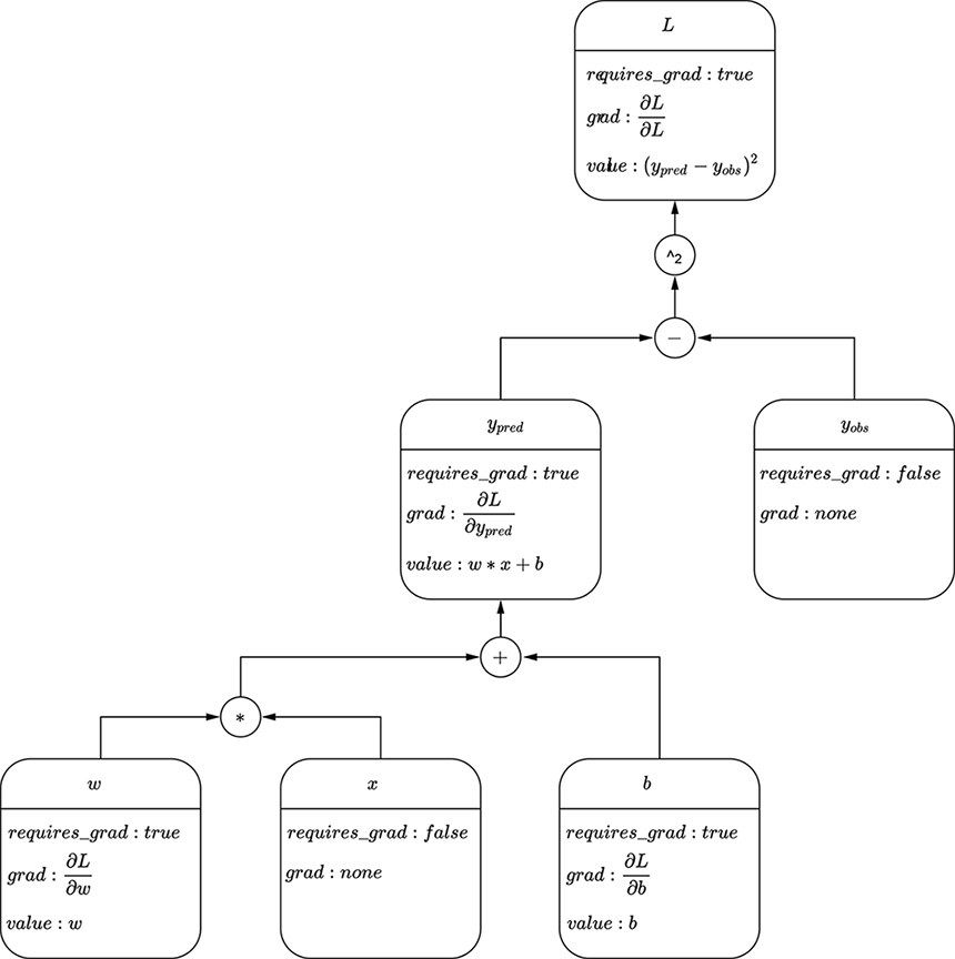
In the PyTorch code in listing 3.1, for this specific model architecture, we computed the gradient using calculus. This approach does not scale to more complex models with millions of weights and perhaps nonlinear complex functions. For scalability, we use an automatic differentiation software library like PyTorch Autograd. Users of the library need not worry about how to compute the gradients—they just construct the model function. Once the function is specified, PyTorch figures out how to compute its gradient through the Autograd technology.
To use Autograd, we explicitly tell PyTorch to track gradients for a variable by setting requires_grad = True when creating the variable. PyTorch remembers a computation graph that is updated every time we create an expression using tracked variables. Figure 3.10 shows an example of a computation graph.
The following listing, which implements a linear model in PyTorch, relies on PyTorch’s Autograd for gradient computation. Note that this method does not require the closed-form gradient.
Listing 3.2 Linear modeling with PyTorch
def update_parameters(params, learning_rate):            ①

  with torch.no_grad():                                  ②
    for i, p in enumerate(params):
      params[i] = p - learning_rate * p.grad

    for i in range(len(params)):
      params[i].requires_grad = True                     ③

x = 10 * torch.randn(N)                                  ④
y  = 1.5 * x + 2.73

y_obs = y + (0.5 * torch.randn(N))                       ⑤

w = torch.randn(1, requires_grad=True)
b = torch.randn(1, requires_grad=True)
params = [b, w]                                          ⑥

for step in range(num_steps):
  y_pred = params[0] + params[1] * x

  mean_squared_error = torch.mean((y_pred - y_obs) ** 2) ⑦

  mean_squared_error.backward()                          ⑧

  update_parameters(params, learning_rate)               ⑨

print("True function: y = 1.5*x + 2.73")
print("Learned function: y_pred = {}*x + {}"
      .format(params[1].data[0], params[0].data.[0]))
① Updates parameters: adjusts the weight, bias along the gradient of error
② Doesn’t track gradients during parameter updates
③ Restores gradient tracking
④ Generates random training input
⑤ Generates training output: applies a simple known function to the input and then adds noise. Let’s see if our learned function matches the known underlying function.
⑥ Our model, initialized with arbitrary parameter values
⑦ The model error is the (squared) difference
between the observed and predicted values.
⑧ Backpropagates: computes the partial
derivatives of the error with respect to
each variable and stores them in the “grad” field within the variable
⑨ Updates parameters using those partial derivatives
The output is as follows:
True function: y = 1.5*x + 2.73
Learned function: y_pred = 1.50059*x + 2.74783
3.5.3 Nonlinear Models in PyTorch
In listings 3.1 and 3.2, we fit a linear model to a data distribution that we know to be linear. From the output, we can see that those models converged to a pretty good approximation of the underlying output function. This is also shown graphically in figure 3.11. But what happens if the underlying output function is nonlinear?
First, listing 3.3 tries to use a linear model on a nonlinear data distribution. As expected (and demonstrated via the output as well as figure 3.12), this model does not do well, because we are using an inadequate model architecture. Further training will not help.
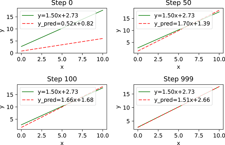
Figure 3.11 Linear approximation of linear data. By step 1,000, the model has more or less converged to the true underlying function.
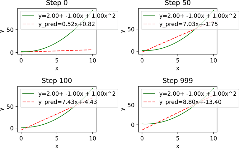
Figure 3.12 Linear approximation of nonlinear data. Clearly the model is not converging to anything close to the desired/true function. Our model architecture is inadequate.
Listing 3.3 Linear approximation of nonlinear data
x = 10 * torch.rand(N, 1)                    ①

y = x**2 - x + 2.0
y_obs = y + (0.5 * torch.rand(N, 1) - 0.25)  ②

w = torch.rand(1, requires_grad=True)
b = torch.rand(1, requires_grad=True)
params = [b, w]
for step in range(num_steps):
  y_pred = params[0] + params[1] * x         ③
  mean_squared_error = torch.mean((y_pred - y_obs) ** 2)
  mean_squared_error.backward()
  update_parameters(params, learning_rate)

print("True function: y = 1.5*x + 2.73")
print("Learned function: y_pred = {}*x + {}"
      .format(params[1].data[0], params[0].data[0]))
① Generates random input training data
② Generates training output: applies a known nonlinear function to the input and then perturbs it with noise
③ Trains a linear model as in listing 3.2
Here is the output:
True function: y=x^2 -x + 2
Learned function: y_pred = 8.79633331299*x + -13.4027605057
Next, listing 3.4 tries a nonlinear model. As expected (and demonstrated via the output as well as figure 3.13), the nonlinear model does well. In real-life problems, we usually assume nonlinearity and choose a model architecture accordingly.
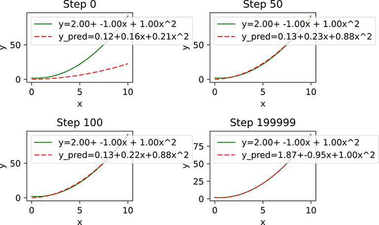
Figure 3.13 If we use a nonlinear model, it more or less converges to the true underlying function.
Listing 3.4 Nonlinear modeling with PyTorch
params = [w0, w1, w2]
for step in range(num_steps):
    y_pred = params[0] + params[1] * x + params[2] * (x**2)
    mean_squared_error = torch.mean((y_pred -y_obs) ** 2)
    mean_squared_error.backward()
    update_parameters(params, learning_rate)

print("True function: y= 2 - x + x^2")
print("Learned function: y_pred = {} + {}*x + {}*x^2"
      .format(params[0].data[0],
              params[1].data[0],
              params[2].data[0]))
Here is the output:
True function: y= 2 - x + x^2
Learned function: y_pred = 1.87116754055+-0.953767299652*x+0.996278882027*x^2
3.5.4 A linear model for the cat brain in PyTorch
In section 2.12.5, we solved the cat-brain problem directly via pseudo-inverse. Now, let’s train a PyTorch model over the same dataset. As expected, the model parameters will converge to a solution close to that obtained by the pseudo-inverse technique this being a simple training dataset); but in the following listing, we demonstrate our first somewhat sophisticated PyTorch model.
Listing 3.5 Our first realistic PyTorch model (solves the cat-brain problem)
X = torch.tensor([[0.11, 0.09], ... [0.63, 0.24]])       ①

X = torch.column_stack((X, torch.ones(15)))              ①
    ②
y = torch.tensor([-0.8, ... 0.37])                       ①

class LinearModel(torch.nn.Module):
    def __init__(self, num_features):
        super(LinearModel, self).__init__()


        self.w = torch.nn.Parameter(                     ③
            torch.randn(num_features, 1))

    def forward(self, X):
        y_pred  = torch.mm(X, self.w)                    ④
        return y_pred

model =  LinearModel(num_features=num_unknowns)

loss_fn = torch.nn.MSELoss(reduction='sum')              ⑤

optimizer = torch.optim.SGD(model.parameters(), lr=1e-2) ⑥

for step in range(num_steps):
    y_pred = model(X)
    loss = loss_fn(y_pred, y)
    optimizer.zero_grad()                                ⑦
    loss.backward()                                      ⑧

    optimizer.step()                                     ⑨

solution_gd = torch.squeeze(model.w.data)
print("The solution via gradient descent is {}".format(solution_gd))
① X, ![]() created (see section 2.12.3) as per equation 2.22 It is easy to verify that the solution to equation 2.22 is roughly w0 = 1, w1 = 1, b = −1. But the equations are not consistent: no one solution perfectly fits all of them. We expect the learned model to be close to y = x0 + x1 − 1.
created (see section 2.12.3) as per equation 2.22 It is easy to verify that the solution to equation 2.22 is roughly w0 = 1, w1 = 1, b = −1. But the equations are not consistent: no one solution perfectly fits all of them. We expect the learned model to be close to y = x0 + x1 − 1.
② Adds a column of all 1s to augment the data matrix X
③ Parameter is a type (subclass) of Torch Tensor suitable for model parameters (weights+bias).
④ Linear model: ![]() = X
= X![]() (X is augmented, and
(X is augmented, and ![]() includes bias)
includes bias)
⑤ Ready-made class for computing squared error loss/
⑥ Ready-made class for updating weights using the gradient of error
⑦ Zeros out all partial derivatives
⑧ Computes partial derivatives via autograd
⑨ Updates the parameters using gradients computed in the backward() step
The output is as follows:
The solution via gradient descent is [ 1.0766 0.8976 -0.9581]
3.6 Convex and nonconvex functions, and global and local minima
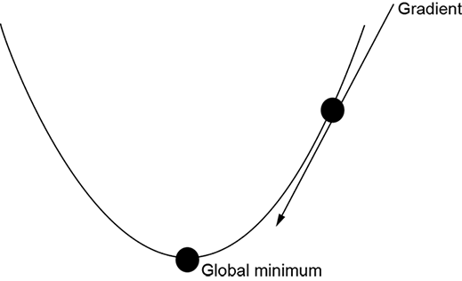
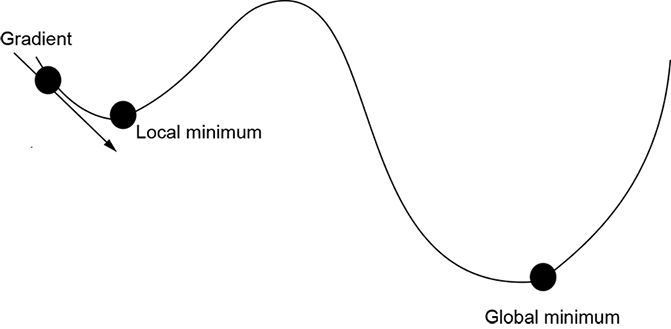
A convex surface (see figure 3.14) has a single optimum (maximum/minimum): the global one.2 Wherever we are on such a surface, if we keep moving along the gradient in parameter space, we will eventually reach the global minimum. On the other hand, on a nonconvex surface, we might get stuck in a local minimum. For instance, in figure 3.14b, if we start at the point marked with the arrowed line indicating a gradient and move downward following the gradient, we will arrive at a local minimum. At the minimum, the gradient is zero, and we will never move out of that point.
(a) A convex function
(b) A nonconvex function
Figure 3.14 Convex vs. nonconvex functions. Convex functions have only a global optimum (minimum or maximum), nolocal optimum. Following the gradient downward is guaranteed to reach the global minimum. Friendly error functions are convex. A nonconvex function has one or more local optima. Following the gradient may reach a local minimum and never discover the global minimum. Unfriendly error functions are nonconvex.
There was a time when researchers put a lot of effort into trying to avoid local minima. Special techniques (such as simulated annealing) were developed to avoid them. However, neural networks typically do not do anything special to deal with local minima and nonconvex functions. Often, the local minimum is good enough. Or we can retrain by starting from a different random point, which may help us escape the local minimum.
3.7 Convex sets and functions
In section 3.6, we briefly encountered convex functions and how convexity tells us whether a function has local minima. In this section, we look at convex functions in more detail. In particular, we learn how to tell whether a given function is convex. We also discuss some important properties of convex functions that will come in handy later—for instance, when we study Jensen’s inequality in probability and statistics, in the appendix. We will mostly illustrate the ideas in 2D space, but they can be easily extended to higher dimensions.
3.7.1 Convex sets
Informally speaking, a set of points is said to be convex if and only if the straight line joining any pair of points in the set lies entirely within the set. For example, if we join any pair of points in the shaded region on the left-hand side of figure 3.15 with a straight line, all points on that line will also be in the shaded region. This is illustrated by points A and B in the figure. The complete set of points in any such region constitutes a convex set.
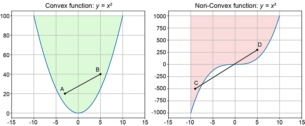
Figure 3.15 Convex and nonconvex sets. The points in the left-hand shaded region form a convex set.The line joining any pair of points in that shaded region lies entirely in the shaded region: for example, AB.The points in the right-hand shaded region form a nonconvex set. For instance, the line joining points C and D passes through a nonshaded region even though both end points belong to a shaded region.
Conversely, a set of points is nonconvex if it contains at least one pair of points whose joining line contains a point not belonging to the set. For instance, the shaded region on the right-hand side of figure 3.15 contains a pair of points C and D whose joining line passes through points not belonging to the shaded region.
The boundary of a convex set is always a convex curve.
3.7.2 Convex curves and surfaces
Consider a function g(x). Let’s pick any two points on the curve y = g(x): A ≡ (x1, y1 = g(x1)) and B ≡ (x2, y2 = g(x2)). Now consider the line segment L joining A and B. From section 2.8.1 (equation 2.12 and figure 2.8), we know that all points C on L can be expressed as a weighted average of the coordinates of A and B, with the sum of weights being 1. Thus, C ≡ (α1x1 + α2x2, α1y1 + α2y2), where α1 + α2 = 1. Compare C with its corresponding point D on the curve, which has the same X coordinate:
D ≡ (α1x1 + α2x2, g(α1x1 + α2x2)).
If and only if g(x) is a convex function, C will always be above D, or
α1y1 + α2y2 = α1g(x1) + α2g(x2) ≥ g(α1x1 + α2x2)
Viewed another way, if we drop a perpendicular to the X-axis from any point on the secant line joining a pair of points on the curve, that perpendicular will cut the curve at a lower point (that is, smaller in its Y-coordinate).
This is illustrated on the left-hand side of figure 3.19 with the function g(x) = x2 known to be convex) and A ≡ (−3,9) and B ≡ (5,25), α1 = 0.3, α2 = 0.7. It can be seen that the weighted average point C on the line lies above the corresponding point on the curve D. The right-hand side illustrates the nonconvex function g(x) = x3, with A ≡ (−8,−512) and B ≡ (5,125), α1 = 0.3, α2 = 0.7. The figure shows one weighted average point (C) on the line joining points A and B on the curve: C lies below point D on the curve, which has the same X-coordinate.
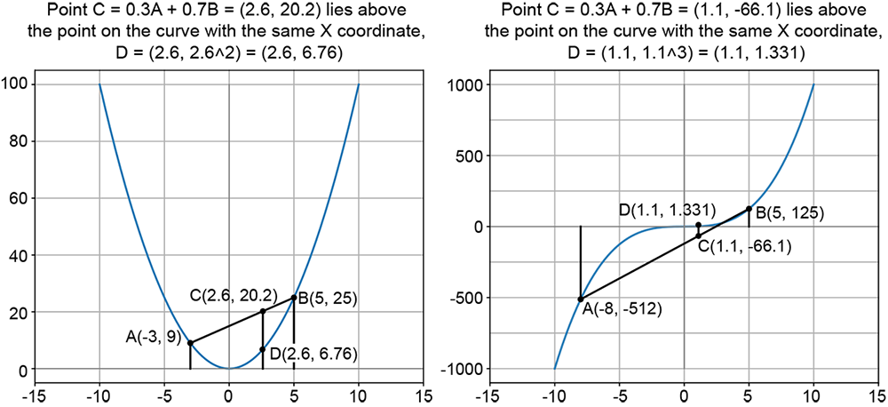
Figure 3.16 Convex and nonconvex curves. A and B are a pair of points on the curve. C = 0.3A + 0.7B is a weighted average of the coordinates of A and B, with weights summing to 1. C lies on the line joining A and B. The left-hand curve is convex: C lies above the corresponding curve point D. The right-hand curve is nonconvex: C lies below the corresponding curve point D.
We need not restrict ourselves to two points. We can take the weighted average of an arbitrary number of points on the curve, with the weights summing to one. The point corresponding to the weighted average will lie above the curve (that is, above the point on the curve with the same X-coordinate). The idea also extends to higher dimensions, as discussed next.
Definition 1
In general, a multidimensional function g(![]() ) is convex if and only if
) is convex if and only if
-
Given an arbitrary set of points on the function surface (curve, if the function is 1D), (
1, g(1)), (2, g(2)), ⋯, (n, g(n)), -
And given an arbitrary set of n weights α1, α2, ⋯, αn that sum to 1 (that is, Σin= 1 αi = 1),
-
The weighted sum of the function outputs exceeds or equals the function output on the weighted sums:
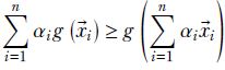
Equation 3.11
A little thought will reveal that definition 1 implies that convex curves always curl upward and/or rightward everywhere. This leads to another equivalent definition of convexity.
Definition 2
In general, a multidimensional function g(![]() ) is convex if and only if
) is convex if and only if
-
A 1D function g(x) is convex if and only if its curvature is positive everywhere:
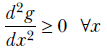
Equation 3.12
-
A multidimensional function g(
) is convex if and only if its Hessian matrix (see section 3.4.2, equation 3.9) is positive semi-definite that is, all the eigenvalues of the Hessian matrix are greater than or equal to zero). This is just the multidimensional analog of equation 3.12.
One subtle point to note is that if the second derivative is negative everywhere or the Hessian is negative semi-definite, the curve or surface is said to be concave. This is different from nonconvex curves, where the second derivative is positive in some places and negative in others. The negative of a concave function is a convex function. But the negative of a nonconvex function is again nonconvex.
A function that curves upward everywhere always lies above its tangent. This leads to another equivalent definition of a convex function.
Definition 3
In general, a multidimensional function g(![]() ) is convex if and only if
) is convex if and only if
-
A function g(x) is convex if and only if all the points on the curve S ≡ (x, g(x)) lie above the tangent line T at any point A on S, with S touching T only at A.
-
A function g(
) is convex if and only if all the points on the surface S ≡ (, g()) lie above the tangent plane T at any point A on S, with S touching T only at A.
This is illustrated in figure 3.17.
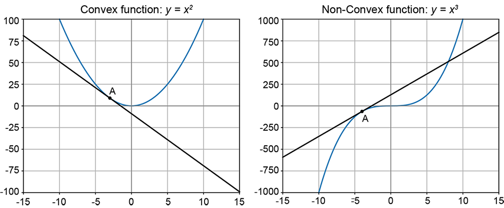
Figure 3.17 The left-hand curve is convex. If we draw a tangent line at any point A on the curve, the entire curve is above the tangent line, touching it only at A. The right-hand cuve is nonconvex: part of the curve lies above the tangent and part of it below.
3.7.3 Convexity and the Taylor series
In section 3.4.1, equation 3.7, we saw the one-dimensional Taylor expansion for a function in the neighborhood of a point x. If we retain the terms in the Taylor expansion only up to the first derivative and ignore all subsequent terms, that is equivalent to approximating the function at x with its tangent at x (see figure 3.17). This is the linear approximation to the curve. If we retain one more term (that is, up to the second derivative), we get the quadratic approximation to the curve. If the second derivative of the function is always positive (as in convex functions), the quadratic approximation to the function will always be greater than or equal to the linear approximation. In other words, locally, the curve will curve so that it lies above the tangent. This connects the second derivative definition (definition 2) with the tangent definition (definition 3) of convexity.
3.7.4 Examples of convex functions
The function g(x) = x2 is convex. The easiest way to verify this is to compute d2g/dx2 = d2x/dx = 2, which is always positive. In fact, any even power of x, g(x) = x2n for an integer n, such as x4 or x6, is convex. g(x) = ex is also convex. This can be easily verified by taking its second derivative. g(x) = logx is concave. Hence, g(x) = −logx is convex.
Multiplication by a positive scalar preserves convexity. The sum of convex functions is also a convex function.
Summary
We would like to leave you with the following mental pictures from this chapter:
-
Inputs for a machine learning problem can be viewed as vectors or, equivalently, points in a high-dimensional feature space. Classification is nothing but separating clusters of points belonging to individual classes in this space.
-
A classifier is can be viewed geometrically as the hypersurface (aka decision boundary) in the high-dimensional feature space, separating the point clusters corresponding to individual classes. During training, we collect sample inputs with known classes and identify the surface that best separates the corresponding points. During inferencing, given an unknown input, we determine which side of the decision boundary this point lies in—this tells us the class.
-
For two-class classifiers (aka binary classifiers), if we plug in the point in the function for the classifier hypersurface, the sign of the corresponding output yields the class.
-
To compute the hypersurface decision boundary that best separates the training data, we first choose a parametric function family to model this surface (for example, a hyperplane for simple problems). Then we estimate the optimal parameter values that best separate the training data, usually in an iterative fashion.
-
To estimate the parameter values that optimally separates the training data, we define a loss function that measures the difference between the model output and the known desired output over the entire training dataset. Then, starting from random initial values, we iteratively adjust the parameter values so that the loss value decreases progressively.
-
At every iteration, the adjustment to the parameter values that optimally reduces the loss is estimated by computing the gradient of the loss function.
-
The gradient of a multidimensional function identifies the direction in the parameter space corresponding to the maximum change in the function. Thus, the gradient of the loss function identifies the direction in which we can adjust the parameters to maximally decrease the loss.
-
The gradient is zero at the maximum or minimum point of a function, which is always a point of inflection. This can be used to recognize when we have reached the minimum. However, in practice, in machine learning we often do an early stop: terminate training iterations when the loss is sufficiently low.
-
A multidimensional Taylor series can be used to create local approximations to a smooth function in the neighborhood of a point. The function is expressed in terms of the displacement from the point, the first-order derivatives (gradient), second-order derivatives Hessian matrix), and so on. This can be used to make higher-accuracy approximations to the change in loss value resulting from a displacement in the parameter space.
-
Loss functions can beconvex or nonconvex. In a convex function, there is no local minimum, only a single global minimum. Hence, gradient descent is guaranteed to converge to the global minimum. A nonconvex function can have both a local and a global minimum. So, gradient-based descent may get stuck in a local minimum.
1 If the change in a quantity such as w is infinitesimally small, we use the symbol dw to denote the change. If the change is small but not infinitesimally so, we use the symbol δw. ↩
2 Although the theory applies to either optimum, maximum or minimum, for brevity’s sake, here we will only talk in terms of the minimum ↩